K. Köhler
Vor etwa einem Jahr wurde im Report 2/73 das ASPSystem in unserer Zeitschrift von H. Rist vorgestellt. Wie in diesem Artikel angekündigt, ist das ASP-Verfahren inzwischen für die dreidimensionale Analyse erweitert worden. Wir erläutern dieses Verfahren im folgenden an einem synthetischen Beispiel von der "Messung" bis zum " Endergebnis".
Um eine dritte Dimension berücksichtigen zu können. dürfen die Schüsse und Geophone nicht wie sonst üblich "eindimensional" entlang einer Geraden angeordnet, sondern sie müssen über eine Fläche verteilt sein. Es genügt für das Analysenprogramm, wenn entweder die Position der Schüsse oder die Position der Geophone oder beide um wenige Meter um die Profilachse streuen. Vier zweckmäßige Meßanordnungen für verschiedene Geländebedingungen hat Prof. Krey im Report 3/74 auf Seite 13 in der Figur 2 vorgestellt.
Für unser Beispiel wurde die in Abb. 1 gezeigte Meßanordnung gewählt. Die Geophonauslage verläuft entlang einer Geraden. Beidseitig der Geophonauslage liegen im Abstand von 50 m abwechselnd die Schußpunkte. Der Geophonabstand und der Anlauf in Profilrichtung betragen ebenfalls 50 m. Die Seismogramme haben je 24 Spuren und die überdeckung ist 24-fach.
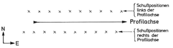
Abb. 1: Skizze des "Meß"-schemas für die Modellrechnung
Figure 1: Sketch of the "recording" scheme for the model data
Mit dieser Meßanordnung wurde das in Abb. 2 perspektivisch dargestellte Laufzeitmodell "vermessen". Es enthält eine Folge von Horizonten im Abstand von jeweils 100 ms. Von diesen Horizonten sind zugunsten der übersichtlichkeit nur einige dargestellt. Um ihren räumlichen Verlauf zu verdeutlichen, wurden sie mit einem Gittermuster überzogen. Wie man sieht, ist die Neigung (Dip) längs des Profils praktisch gleich Null. Quer zum Profil ist die Neigung oberhalb 0,5 s gleich Null. Unterhalb 1 s ist am Profilanfang keine Querneigung vorhanden. Zur Profilmitte hin fortschreitend ist ein zunehmendes Einfallen nach Norden bemerkbar, das bis auf 7,5 ms/25 m anwächst. Es nimmt dann langsam wieder ab und kippt schließlich in ein entgegengesetztes Einfallen von 5 msl 25 m nach Süden um. Von der Laufzeit 0,5 s bis zur Laufzeit 1 s wird der Dip linear interpoliert.
Die Meßanordnung bewirkt, daß die Signale in den Seismogrammen, bei denen die zugehörigen Schüsse nördlich der Profilachse liegen, je nach dem jeweiligen Querdip, eine geringe Zeitverschiebung gegenüber den Signalen aufweisen, bei denen die zugehörigen Schüsse südlich der Profilachse liegen. Daraus läßt sich nach Durchführung der dynamischen Korrektur der Querdip bereits ableiten. Der Computer arbeitet jedoch etwas anders. Er vergleicht nicht die Laufzeiten benachbarter Einzelspuren, sondern die Zeiten jeder Einzelspur mit einer mitgeführten Referenzspur. Diese Referenzspur wird jeweils von einem Untergrundpunkt zum nächsten entsprechend dem Längsdip vorhergesagt und dann aufgrund der Meßwerte für den neuen Untergrundpunkt etwas verbessert. Die Referenzspur ist bekanntlich die Spur, mit der alle Spuren für jeden Untergrundpunkt der Reihe nach verglichen werden.
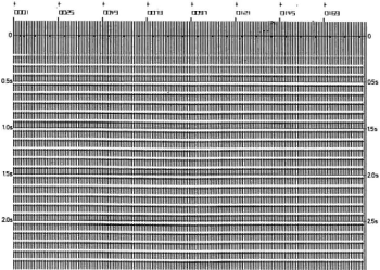
Abb.3: Stapelsektion
Figure 3: Stacked section
Nach der dynamischen Korrektur und der Kompensation des Dips ist zu erwarten, daß die Laufzeiten der Signale auf einer Spur mit den Laufzeiten auf der Referenzspur übereinstimmen. Ist das nicht der Fall, wird aus der Zeitdifferenz eine Änderung im Geschwindigkeitsgesetz, eine Änderung des Dip in Profilrichtung und eine Änderung des Dip quer zum Profil abgeleitet.
3D-ASP-Analysis
About one year ago the ASP-system was introduced by H. Rist in our magazine Report 2/73. As was announced in this article, the ASP-system has in the meantime been extended to 3-dimensional analysis. We explain this process trom "survey" to "result" as follows using a synthetic example.
In order to take into consideration a third dimension, the shots and geophones are not arranged, as usual, in one dimension along a straight line, but they are spread over a plane. It is sufficient for the analysis program if either the position of the shots or of the geophones or both are spread a few meters off the axis of the line. Professor Krey introduced 4 suitable survey arrangements for different field conditions in Report 3/74 on page 13, figure 2.
For our example the survey arrangement shown in figure 1 was chosen. The geophone spread runs along a straight line. The shotpoints lie alternatelyon either side of the geophone spread with an offset of 50 m. The geophone spacing and the in-line offset are also 50 m. The seismograms have 24 traces each and the coverage is 24 fold.
With this survey arrangement the travel time model, outlined perspectively in figure 2, has been "surveyed". It contains aseries of horizons with a spacing of 100 ms each. Of these horizons only a few are outlined for the benefit of clarity; in order to illustrate their spatial course they were covered with a grid pattern.
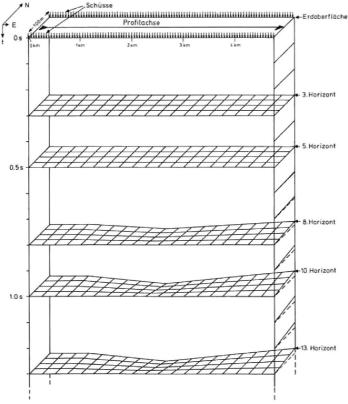
Abb. 2: Lotzeitmodell, an dem die 3D-ASP-Analyse getestet wurde. Es ist nur eine Auswahl der Horizonte abgebildet. Die ausgelassenen Horizonte sind am rechten Rand des Modells angedeutet.
Figure 2: Model of the two-way travel times after dynamic correction, as they were used in the test of the 3D-ASP analysis. Only a selection of the horizons is shown. The missing horizons are indicated at the right side of the model.
One can see that the in-line dip is practically zero. Perpendicular to the line the dip above 0.5 s is practically zero. Below 1 s there is no cross dip at the beginning of the line. Progressively toward the middle of the line an increasing dip to the north is noticeable which increases up to 7,5 ms/25 m. It decreases slowly again and finally turns in an opposite dip of 5 ms per 25 m to the south. From the travel time 0.5 s to 1 s the dip has been interpolated linearly.
The signals in the seismograms from the shot points north of the line axis show, depending on the specific cross dip, a short time difference to the signals in the seismograms from the relevant shots south of the line. Thus, one can already derive the cross dip after having carried out the dynamic corrections. But the computer works in a different way. He does not compare the travel times of single neighbouring traces but the times of each single trace with a reference trace.
Abb.4: Darstellung des Querdips entlang ausgewählter Laufzeitkurven. Nach unten aufgetragene Marken bedeuten ein Einfallen zur rechten Seite des Profils -im vorliegenden Fall also nach Süden. (Im doppelten Maßstab der Abb.3, 5 und 6, um das Ablesen zu erleichtern)
Figure 4: Presentation of the cross dip along selected travel time curves. Marks plotted below these curves represent a dip to the right side of the line - i. e. in the present case to the south.
∇
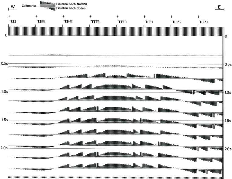
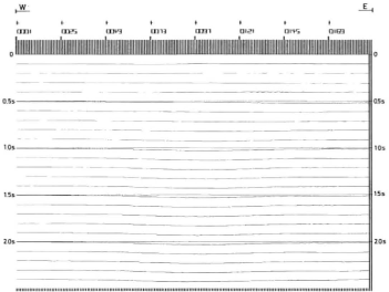
Abb.5: Darstellung des Dips längs des Profils durch Linien, die dem Dip folgen.
Figure 5: Presentation of the dip in the direction of the line by means of curves following the dip.
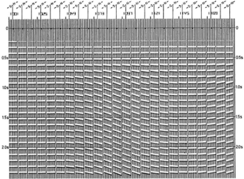
Abb.6: Darstellung des Querdips durch kurze Querprofile.
Figure 6: Presentation of the cross dip by means of shorl cross sections.
Diese drei Werte können natürlich nicht schon nach der Bearbeitung einer einzelnen Spur zuverlässig ermittelt werden, weil dabei aus einer einzigen Messung drei Unbekannte bestimmt werden. Diese Ableitung wird jedoch für jede neu zu analysierende Spur wiederholt und dadurch das Ergebnis iterativ verbessert. Aufgrund der riesigen Anzahl von Spuren, die zu einem Profil gehören, wird schließlich ein zuverlässiges Ergebnis erreicht.
Von den Ergebnissen der 3D-ASP-Analyse sollen hier nur die gestapelte Sektion und die Dip-Darstellungen gezeigt werden. Die gestapelte Sektion ist in Abb. 3 zu sehen. Die Abb. 4 zeigt den Querdip. Dieses Dip-Profil enthält Angaben über den Querdip längs vorgewählter Laufzeitkurven, im vorliegenden Fall für die konstanten Laufzeiten 350 ms, 550 ms, 750 ms usw. in Differenzen von 200 ms bis 2350 ms. Bei diesen Laufzeiten sind horizontale Striche je nach dem Vorzeichen des Dips über oder unter der Laufzeitmarke aufgetragen. Jeder Strich bedeutet einen Dip von 1 Sample/Spurabstand (Samplingrate = 2 ms). Zusätzlich sind an jedem Untergrundpunkt "Säulen" mit Meßmarken (Querstriche) aufgesetzt. Der Abstand der Meßmarken untereinander entspricht 0,1 Sample/Spurabstand. Die jeweilige Summe gibt den Querdip bei der entsprechenden Laufzeit an.
Die beschriebene Art der Darstellung des Querdips liefert im vorliegenden Beispiel ein zahlenmäßig auswertbares Bild der Neigungsverhältnisse. Man erkennt, wie im unteren Teil der Sektion sich der Querdip entlang des Profils ändert. Der maximale Querdip ist mit 3,75 Samples/ Spurabstand, entsprechend den Neigungsverhältnissen am Modell, richtig wiedergegeben (die Sampling Rate betrug in diesem Fall 2 ms). Der Dip längs des Profils wäre in dieser Darstellungsart nicht zu erkennen, da er maximal nur 0,0625 samples/Spurabstand beträgt.
Die in der Abbildung 4 gezeigte Darstellung des Dips ist zwar zahlenmäßig auswertbar, aber nicht sehr anschaulich. Um den Dip anschaulicher zu machen, werden deshalb noch zwei weitere Darstellungsarten in den Abbildungen 5 und 6 gezeigt. In Abb. 5 ist der Dip längs des Profils durch Linien dargestellt, deren Verlauf dem Dip folgt. In Abb. 6 ist der Querdip durch eine Serie von kurzen Querprofilen in N/S-Richtung verdeutlicht. Die mittleren Spuren jedes dieser Querprofile sind jeweils die an der entsprechenden Stelle gebildeten Stapelspuren. Entlang dem gemessenen Querdip sind aus diesen Spuren die übrigen Spuren der kurzen Querprofile extrapoliert worden. Ein räumliches Bild würde man erhalten, wenn man die Querprofile einzeln ausschneiden und um 90° nach links drehen würde.
In diesem Artikel ist viel von den verschiedenen Möglichkeiten der Darstellung geschrieben worden. Neben der Analyse der Daten ist die Darstellung der Ergebnisse tatsächlich ein zentrales Problem ; sie wird dadurch so kompliziert, daß man eine räumliche Struktur auf einem Blatt Papier, also in nur zwei Dimensionen, abbilden muß. Je nach dem Verwendungszweck wird die eine oder andere Art der Darstellung zu empfehlen sein. Bei Bedarf können außer den gezeigten Darstellungsarten auch noch weitere angeboten werden.
In einem der nächsten Reports soll das dreidimensionale ASP-Verfahren an einem gemessenen Profil demonstriert werden. Dabei kann natürlich nicht dieselbe extreme Genauigkeit wie bei der Analyse eines synthetischen Profiles erwartet werden. Es ist aber damit zu rechnen, daß die 3D-ASP-Analyse die Interpretation der bearbeiteten Profile wesentlich stützen und verfeinern wird.
This reference trace is predicted from one subsurface point to the next one, according to the longitudinal dip, and then it is updated with the differences to the measured signal values for the new subsurface point. The reference trace is, as you know, the trace with which all traces for each subsurface point are compared and updated continuously. After the dynamic correction and the dip compensation one can expect that the travel times of this signals on one trace correspond to the signal times of the reference trace. If this is not the case there will be, derived from the time differencies, a change in the velocity function, a change of the in-line dip and a change of the cross dip. These three values of course cannot be detected reliably after processing of one single trace because 3 unknown quantities are being determined from one single measurement. But this deduction is being repeated for each new analyzed trace and through this the result is improved by iteration. Because of the enormous number of traces belonging to one line a reliable result is finally achieved.
Of the results of the 3D-ASP-analysis only the stacked section and the dip displays shall be shown. The stacked section you can see in figure 3. Figure 4 shows the cross dip. This dip section contains information about the cross dip along pre-selected travel time curves, in our case for the constant travel times 350 ms, 550 ms, 750 ms a.s.o., in steps from 200 ms, to 2350 ms. At each of these travel times, horizontal lines -depending on the sign of the dip, either above or below the time marker lines -are plotted. Each line corresponds to the dip of 1 sampie per trace interval (sampling rate 2 ms). Additionaly at each subsurface point "columns" with measuring marks (serifs) are set up. The spacing between each of these measuring marks corresponds to 0.1 sampie per trace spacing. The respective sum gives the cross dip at the corresponding travel time.
Our type of display of the cross dip supplies in this specific example a numerically interpretable design of the dip situation. One can see how in the lower part of the section the cross dip changes along the line. The maximum cross dip is, with 3.75 sampies per trace spacing, correctly represented corresponding to the dip situation in the model. The in-line dip would not have been detectable in this type of display because it only adds up to a maximum of 0.0625 sam pies per trace spacing.
The presentation of the dip in figure 4 is admittedly numerically interpretable but not very illustrative. To make the dip more clear two further types of display are shown in figures 5 and 6. In figure 5 the in-li ne dip is represented by lines whose course follows the dip. In figure 6 the cross dip is illustrated through aseries of short cross lines in N/S direction. The middle traces of each of these cross lines are the respective stack traces. From these traces the other traces of the short cross lines were extrapolated along the measured cross dip. A spatial picture would be obtained if the cross lines were cut out singly and turned 90° to the left.
In this article a lot has been written about the different display possibilities. Besides the data analysis the display of results is actually a central problem ; it becomes so complicated because one has to represent a spatial struture on a sheet of paper which means only in two dimensions. Depending on the application either one or the other type of display will be recommended. By request, in addition to the types of display shown, further on es can be offered.
In one of the next reports the 3-dimensional ASP-system will be demonstrated on a surveyed section. In this, of course, one cannot expect the same extreme accuracy as in the analysis of a synthetic section. But it may be expected that the 3D-ASP-analysis will substantially support and refine the interpretation of processed sections.